Fisher’s Ideal Index Number

Management > Managerial Statistics > Index Number By Fisher’s Method

Laspeyre’s method is based on fixed weights of the base year. For price index base year’s quantities are used as weights. Paasche’s method is based on fixed weights of the current year. For price index, current year’s quantities are used as weights. Fisher has suggested a geometric mean of the two indices (Laspeyres and Paasche) mentioned above so as to take into account the influence of both the periods, i.e., current as well as base periods.  Thus Fisher’s Method is a geometric mean of Laspeyre’s index and Passche’s index.

Price Index by Fisher’s Method:

Steps involved:

1. Denote prices of the commodity in the current year as P1 its quantity consumed in that year by Q1.
2. Denote prices of the commodity in the base year as P0 and its quantity consumed in that year by Q0.
3. Find the quantities P0Q0, P1Q0, P0Q1, and p1Q1 for each commodity.
4. Find the sum of each column of P0Q0, P1Q0 , P0Q1, and p1Q1 denote the sums by ∑ P0Q0, ∑ P1Q0, ∑ P0Q1, and ∑ P1Q1 respectively.
5. Find the Laspeyre’s Price index number
6. Find the Paasche’s Price index number
7. To find the Fisher’s index number calculate the geometric mean of Laspeyre’s index and Passche’s index.

Laspeyre’s price index

LP₀₁ = (∑ P₁ x Q₀) / ( ∑ P₀ x Q₀) × 100

Paasche’s index

PP₀₁ = (∑ P₁ x Q₁) / ( ∑ P₀ x Q₁ ) × 100

Fisher’s index number

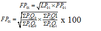
Example – 01:

Compute Price index by Dorbish and Browley’s Method from the following data.

Commodity	Base Year		Current Year
	Price	Quantity	Price	Quantity
A	3	25	5	28
B	1	50	3	60
C	2	30	1	30
D	5	15	6	12

Solution:

Commodity	Base Year		Current Year
	P0	Q0	P1	Q1	P0Q0	P1Q0	P0Q1	P1Q1
A	3	25	5	28	75	125	84	140
B	1	50	3	60	50	150	60	180
C	2	30	1	30	60	30	60	30
D	5	15	6	12	75	90	60	72
Total					∑P0Q0=260	∑P1Q0=395	∑P0Q1=264	∑P1Q1=422

Lapeyre’s Price Index = LP₀₁ = (∑ P₁ x Q₀) / (∑ P₀ x Q₀) × 100

LP₀₁ = (395 / 260) × 100

LP₀₁ = 151.92

Paasche’s Price Index = PP₀₁ = (∑ P₁ x Q₁) / (∑ P₀ x Q₁) × 100

PP₀₁ = (422 / 264) × 100

PP₀₁ = 159.85

Direct Calculation:

Fisher’s price index is 155.89

Quantity Index by Fisher’s Method:

Steps involved:

1. Denote prices of the commodity in the current year as P1 its quantity consumed in that year by Q1.
2. Denote prices of the commodity in the base year as P0 and its quantity consumed in that year by Q0.
3. Find the quantities P0Q0, P1Q0, P0Q1, and p1Q1 for each commodity.
   Find the sum of each column of P0Q0, P1Q0 , P0Q1, and p1Q1 denote the sums by ∑ P0Q0, ∑ P1Q0, ∑ P0Q1, and ∑ P1Q1 respectively.
4. Find the Laspeyre’s Quantity index number
5. Find the Paasche’s Quantity index number
6. To find the Fisher’s index number calculate the geometric mean of Laspeyre’s index and Passche’s index.

Laspeyre’s quantity index

LQ₀₁ = (∑ Q₁ x P₀) / ( ∑ Q₀ x P₀) × 100

Paasche’s quanity index

PQ₀₁ = (∑ Q₁ x P₁) / ( ∑ Q₁ x P₀ ) × 100

Fisher’s quantity index number

Example – 02:

Compute Price index by Dorbish and Browley’s Method from the following data.

Commodity	Base Year		Current Year
	Price	Quantity	Price	Quantity
A	3	25	5	28
B	1	50	3	60
C	2	30	1	30
D	5	15	6	12

 

Commodity	Base Year		Current Year
	P0	Q0	P1	Q1	Q0P0	Q1P0	Q0P1	P1Q1
A	3	25	5	28	75	84	125	140
B	1	50	3	60	50	60	150	180
C	2	30	1	30	60	60	30	30
D	5	15	6	12	75	60	90	72
Total					∑P0Q0=260	∑P1Q0=264	∑P0Q1=395	∑P1Q1=422

Laspeyre’s Quantity Index = LQ₀₁ = (∑ Q₁ x P₀) / (∑ Q₀ x P₀) × 100

LQ₀₁ = (264 / 260) × 100

LQ₀₁ = 101.54

Pasche’s Quantity Index = PQ₀₁ = (∑ Q₁ x P₁) / ( ∑ Q₀ x P₁) × 100

PQ₀₁ = (422 / 395) × 100

PQ₀₁ = 106.84

Direct Calculation:

Fisher’s quantity index is 104.16

Advantages of Fisher’s Method:

• It is free from bias. It reduces the influence of high and low values of the data.
• This method considers values of both, the current year and the base year.
• Fisher’s index lies between the other two indexes.  It is referred to as an “ideal” index because it correctly predicts the expenditure index and it satisfies both the time reversal test as well as factor reversal test.

Disadvantages of Fisher’s Method:

• It is tedious and time-consuming.
• As the data of the current year and the base year is required, the data collection is costly and time-consuming.

Previous Topic: Dorbish and Browley’s Method

Next Topic: Marshall Edgeworth Method

Management > Managerial Statistics > Index Number By Fisher’s Method